Courses & Projects by Rob Marano
Notes for Week 3
← back to syllabus ← back to notes
Topics
- Verilog: Parameterization; Built-in primitives; User-defined primitives; Dataflow modeling
- Stored Program Concept
- History of computer architecture and modern advancements
Topics Deep Dive
More on Verilog
Parameterize Your Verilog Code
Parameters are fundamental for creating reusable and configurable hardware designs. They allow you to define constants that can be modified at compile time, influencing the behavior and structure of your modules. Think of them as global variables within a module’s scope, but with the crucial difference that they are typically resolved before simulation.
Let’s break down how to use parameters effectively in SystemVerilog.
1. Declaring Parameters:
You declare a parameter using the parameter keyword. The basic syntax is:
parameter [data_type] parameter_name = value;
data_type: Specifies the data type of the parameter. Common types include integer, real, time, and enumerated types. If omitted, the type defaults to integer.parameter_name: The name you give to your parameter. Follow standard naming conventions (typically uppercase for parameters).value: The constant value assigned to the parameter. This value can be a constant expression.
Some examples:
parameter WIDTH = 8; // An 8-bit wide value
parameter DEPTH = 256; // A depth value
parameter REAL_VAL = 3.14159; // A real value
parameter logic [7:0] DEFAULT_VALUE = 8'hAA; // An 8-bit logic value
parameter enum { STATE_IDLE, STATE_READ, STATE_WRITE } STATE = STATE_IDLE; // Enumerated type
2. Using Parameters:
Once declared, you can use parameters anywhere within the module where a constant value is required. This includes:
- Module Instantiations: Crucially, parameters allow you to customize module instances.
- Array Sizes: Defining the dimensions of arrays.
- Loop Boundaries: Specifying the limits of for loops.
- Case Statements: Using parameters in case expressions.
- Expressions: Including parameters in arithmetic and logical operations.
For example, a parameterized adder using behavioral modeling
module adder #(parameter WIDTH = 8) (
  input logic [WIDTH-1:0] a,
  input logic [WIDTH-1:0] b,
  input logic cin,
  output logic [WIDTH-1:0] sum,
  output logic cout
);

  assign {cout, sum} = a + b + cin;

endmodule
Using the adder in other modules, like a test bench.
// code below would be in a test bench or another module's definition.
// Instantiating the adder with different widths:
adder #(.WIDTH(16)) adder16 (
  .a(data_a),
  .b(data_b),
  .cin(carry_in),
  .sum(sum16),
  .cout(carry_out)
);

adder adder8 ( // Using the default WIDTH = 8
  .a(data_c),
  .b(data_d),
  .cin(carry_in2),
  .sum(sum8),
  .cout(carry_out2)
);
3. Overriding Parameters:
The real power of parameters comes from the ability to override their values during module instantiation. This is done using the #(.parameter_name(value)) syntax, as shown in the adder example above. This allows you to reuse the same module with different configurations without modifying the module’s source code.
4. Local Parameters:
SystemVerilog also provides the keyword localparam. These are similar to parameters but cannot be overridden during instantiation. They are strictly local to the module in which they are defined. Use localparam for constants that should not be changed externally.
localparam DELAY = 2; // A delay value that should not be modified from outside
Key Advantages of Using Parameters:
- Reusability: Create generic modules that can be adapted to different needs.
- Configurability: Easily change the behavior and structure of your designs without rewriting code.
- Maintainability: Modifications are localized to the parameter declaration, reducing the risk of errors.
- Readability: Using meaningful parameter names makes your code easier to understand.
Best Practices:
- Use uppercase for parameter names.
- Provide default values for parameters.
- Document your parameters clearly.
- Use meaningful names that reflect the parameter’s purpose.
Programmatically Generate Circuits
Generate blocks provide a mechanism for creating multiple instances of modules or code blocks based on compile-time conditions or loop iterations. This is essential for designing regular structures like arrays of processing elements, memory banks, or replicated logic. genvar is a special variable used exclusively within generate blocks as an index or iterator.
1. The genvar Keyword:
genvar declares an integer variable that is used as a loop counter or index within a generate block. It’s crucial to understand that genvar is not a regular variable; it exists only during the elaboration phase (before simulation) and is used to generate hardware instances. You cannot use a genvar outside of a generate block.
genvar i; // Declaring a genvar
2. The generate Block:
The generate block encloses the code that you want to replicate or conditionally instantiate. There are three main types of generate constructs:
forloop generate: Used for repetitive instantiation.if-elsegenerate: Used for conditional instantiation.casegenerate: Used for multi-conditional instantiation (similar to a case statement).
3. for Loop Generate:
This is the most common type. It’s used to create multiple instances of a module or block of code.
generate
  for (genvar i = 0; i < N; i++) begin : instances // 'instances' is a generate block name (important!)
    // Inside the loop, 'i' is used to create unique instances.
    adder #( .WIDTH(WIDTH) ) adder_inst (
      .a(data_a[i*WIDTH+:WIDTH]), // Using 'i' to index into a wider data bus
      .b(data_b[i*WIDTH+:WIDTH]),
      .cin(carry_in[i]),
      .sum(sum[i*WIDTH+:WIDTH]),
      .cout(carry_out[i])
    );
  end
endgenerate
begin : block_name: Giving a name to the generate block is essential, especially for hierarchical referencing and debugging.i*WIDTH+:WIDTH: This is a common pattern for indexing into a wider data bus. It creates slices of thedata_aanddata_bsignals based on thegenvari.- Hierarchical Referencing: You can access instances created within the generate block using hierarchical names, for example,
instances[0].adder_inst.sum.
4. if-else Generate:
This construct allows you to conditionally instantiate different blocks of code based on a compile-time condition.
generate
  if (ENABLE_ADDER) begin : adder_block
    adder #( .WIDTH(WIDTH) ) adder_inst (
      .a(data_a),
      .b(data_b),
      .cin(carry_in),
      .sum(sum),
      .cout(carry_out)
    );
  end else begin : multiplier_block
    multiplier #( .WIDTH(WIDTH) ) multiplier_inst (
      .a(data_a),
      .b(data_b),
      .prod(product)
    );
  end
endgenerate
5. case Generate:
Similar to if-else, but for multiple conditions.
generate
  case (OPERATION)
    ADD: begin : add_block
      // ... instantiation for addition ...
    end
    SUBTRACT: begin : sub_block
      // ... instantiation for subtraction ...
    end
    default: begin : default_block
      // ... default instantiation ...
    end
  endcase
endgenerate
Important Considerations:
- Compile-Time Evaluation: Generate blocks and
genvarstatements are evaluated during the elaboration phase, not during simulation. This means the conditions and loop iterations must be known at compile time. You cannot use run-time signals to control generate blocks. - Generate Block Names: Always name your generate blocks using
begin : block_name. This is crucial for hierarchical referencing and debugging. - Scope:
genvarvariables are only visible within thegenerateblock. - No Assignments to
genvars: You cannot assign values to agenvarinside thegenerateblock. They are automatically incremented inforloops.
For example, Parameterized Memory Array:
module memory_array #(
  parameter DEPTH = 256,
  parameter WIDTH = 8
) (
  // ... ports ...
);

  genvar i;
  generate
    for (i = 0; i < DEPTH; i++) begin : memory_instances
      memory_cell #( .WIDTH(WIDTH) ) mem_cell (
        // ... connections ...
      );
    end
  endgenerate

endmodule
This example creates an array of DEPTH memory cells, each of WIDTH bits.
Conclusion Using genvar and generate
By mastering generate blocks and genvars, you can create highly parameterized and reusable hardware designs, significantly improving your productivity and code maintainability. Now, let’s put this knowledge into practice with some exercises!
Let’s create a variable bit length Register File
Step 1 — The D flip-flop with reset and enable signals:
The dff module:
module dff (
  input logic clk,
  input logic rst,
  input logic enable,
  input logic d,
  output logic q
);

  always_ff @(posedge clk) begin
    if (rst) begin
      q <= 0; // Synchronous reset
    end else if (enable) begin
      q <= d; // Data is loaded only when enable is high
    end
  end

endmodule
The test bench for the dff module:
// Testbench to demonstrate the d_flip_flop
module d_flip_flop_tb;
  logic clk;
  logic rst;
  logic enable;
  logic d;
  logic q;

  d_flip_flop dut (
    .clk(clk),
    .rst(rst),
    .enable(enable),
    .d(d),
    .q(q)
  );

  // Clock generation
  initial begin
    clk = 0;
    forever #5 clk = ~clk; // 10ns period
  end

  // Test sequence
  initial begin
    rst = 1;
    enable = 0;
    d = 0;

    #10 rst = 0; // Release reset

    d = 1;
    enable = 1;
    #10; // q should now be 1

    d = 0;
    enable = 1;
    #10; // q should now be 0

    enable = 0; // Disable the flip-flop
    d = 1;      // Change d, but q should remain unchanged
    #10;       // q should still be 0

    enable = 1; // Enable again
    #10;       // q should now be 1

    $display("Final value of q: %b", q);
    $finish;
  end

endmodule
Step 2 — The Register
The register module:
module register #(
  parameter WIDTH = 8 // Default width of 8 bits
) (
  input logic clk,
  input logic rst,
  input logic enable,
  input logic [WIDTH-1:0] d, // Data input, parameterized width
  output logic [WIDTH-1:0] q // Data output, parameterized width
);

  // Array of D flip-flops to form the register
  logic [WIDTH-1:0] q_internal; // Internal storage for the register

  genvar i;
  generate
    for (i = 0; i < WIDTH; i++) begin : flip_flops
      dff flip_flop_inst (
        .clk(clk),
        .rst(rst),
        .enable(enable),
        .d(d[i]),      // Connecting individual bits of d
        .q(q_internal[i]) // Connecting individual bits of q_internal
      );
    end
  endgenerate

  assign q = q_internal; // Assign the internal storage to the output

endmodule
The test bench for the register module:
// Testbench for the parameterized register
module register_tb;
  logic clk;
  logic rst;
  logic enable;
  logic [7:0] d; // 8-bit data for default instantiation
  logic [7:0] q;

  // Instantiating the register with the default width (8 bits)
  register reg8 (
    .clk(clk),
    .rst(rst),
    .enable(enable),
    .d(d),
    .q(q)
  );

  // Instantiating the register with a different width (16 bits)
  logic [15:0] d16;
  logic [15:0] q16;
  register #( .WIDTH(16) ) reg16 ( // Parameter override
    .clk(clk),
    .rst(rst),
    .enable(enable),
    .d(d16),
    .q(q16)
  );


  // Clock generation
  initial begin
    clk = 0;
    forever #5 clk = ~clk;
  end

  // Test sequence
  initial begin
    rst = 1;
    enable = 0;
    d = 8'hAA; // Example data for 8-bit register
    d16 = 16'hBEEF; // Example data for 16-bit register

    #10 rst = 0;  // Release reset
    enable = 1;

    #10 d = 8'h55; // Change data for 8-bit register
    #10 d16 = 16'hDEAD; // Change data for 16-bit register

    #10 enable = 0; // Disable

    #10 enable = 1; // Enable again

    #10 $display("8-bit Register q: %h", q); // Should be 55
    #10 $display("16-bit Register q16: %h", q16); // Should be DEAD

    $finish;
  end

endmodule
Step 3 — The Register File
The register_file module:
module register_file #(
  parameter DEPTH = 8,  // Number of registers (default 8)
  parameter WIDTH = 8   // Width of each register (inherited or specified)
) (
  input logic clk,
  input logic rst,
  input logic enable,

  input logic [$log2(DEPTH)-1:0] write_addr, // Write address
  input logic [WIDTH-1:0] write_data,      // Write data
  input logic write_en,                  // Write enable

  input logic [$log2(DEPTH)-1:0] read_addr1, // Read address 1
  output logic [WIDTH-1:0] read_data1,     // Read data 1

  input logic [$log2(DEPTH)-1:0] read_addr2, // Read address 2
  output logic [WIDTH-1:0] read_data2      // Read data 2
);

  // Array of registers
  register #( .WIDTH(WIDTH) ) registers [DEPTH]; // Parameterized register instances

  genvar i;
  generate
    for (i = 0; i < DEPTH; i++) begin : register_instances
      registers[i] (
        .clk(clk),
        .rst(rst),
        .enable(enable),
        .d( (write_en && (write_addr == i)) ? write_data : '0 ), // Conditional write
        .q() // Output not directly connected within the array
      );
    end
  endgenerate

  // Read logic (combinational) - Two independent read ports
  assign read_data1 = registers[read_addr1].q; // Hierarchical access to register output
  assign read_data2 = registers[read_addr2].q; // Hierarchical access to register output

endmodule
The test bench for the register_file module:
// Testbench for the parameterized register file
module register_file_tb;
  logic clk;
  logic rst;
  logic enable;

  logic [2:0] write_addr; // 8 registers so 3 bits for address
  logic [7:0] write_data;
  logic write_en;

  logic [2:0] read_addr1;
  logic [7:0] read_data1;

  logic [2:0] read_addr2;
  logic [7:0] read_data2;

  register_file rf (
    .clk(clk),
    .rst(rst),
    .enable(enable),
    .write_addr(write_addr),
    .write_data(write_data),
    .write_en(write_en),
    .read_addr1(read_addr1),
    .read_data1(read_data1),
    .read_addr2(read_addr2),
    .read_data2(read_data2)
  );

  // Clock generation
  initial begin
    clk = 0;
    forever #5 clk = ~clk;
  end

  // Test sequence
  initial begin
    rst = 1;
    enable = 0;
    write_en = 0;

    #10 rst = 0;
    enable = 1;

    write_addr = 3'h3;
    write_data = 8'hAA;
    write_en = 1;
    #10 write_en = 0;

    write_addr = 3'h5;
    write_data = 8'h55;
    write_en = 1;
    #10 write_en = 0;

    read_addr1 = 3'h3;
    read_addr2 = 3'h5;

    #10;

    $display("Read Data 1 (addr 3): %h", read_data1); // Should be AA
    $display("Read Data 2 (addr 5): %h", read_data2); // Should be 55

    $finish;
  end

endmodule
How about counters?
Simple Counter
The counter module:
module counter #(
  parameter WIDTH = 8 // Default width of 8 bits
) (
  input logic clk,
  input logic rst,
  input logic enable,
  output logic [WIDTH-1:0] count
);

  logic [WIDTH-1:0] count_internal; // Internal storage for the counter

  always_ff @(posedge clk) begin
    if (rst) begin
      count_internal <= '0; // Reset to 0
    end else if (enable) begin
      count_internal <= count_internal + 1; // Increment on rising clock edge when enabled
    end
  end

  assign count = count_internal; // Assign internal value to output

endmodule
The test bench for the counter module:
// Testbench for the counter
module counter_tb;
  logic clk;
  logic rst;
  logic enable;
  logic [7:0] count; // 8-bit count for default instantiation

  // Instantiate the counter (default 8-bit width)
  counter counter_8bit (
  .clk(clk),
  .rst(rst),
  .enable(enable),
  .count(count)
  );

  // Instantiate a 16-bit counter to test parameter override
  logic [15:0] count_16bit;
  counter #(16) counter_16bit_inst ( // Override WIDTH to 16
  .clk(clk),
  .rst(rst),
  .enable(enable),
  .count(count_16bit)
  );


  // Clock generation
  initial begin
    clk = 0;
    forever #5 clk = ~clk; // 10ns period
  end

  // Test sequence
  initial begin
    rst = 1;
    enable = 0;

    #10 rst = 0; // Release reset
    enable = 1;

    #10;      // count should be 1 (8-bit) and 1 (16-bit)
    #10;      // count should be 2 (8-bit) and 2 (16-bit)
    #10;      // count should be 3 (8-bit) and 3 (16-bit)

    $display("8-bit Count: %h", count);      // Should be 3
    $display("16-bit Count: %h", count_16bit); // Should be 3

    // Test overflow for 8-bit counter
    repeat (253) @(posedge clk); // Count up to 255
    #10;
    $display("8-bit Count (Overflow): %h", count); // Should be FF (255)
    #10;
    $display("8-bit Count (After Overflow): %h", count); // Should be 00 (wrapped around)

    // Test overflow for 16-bit counter
    repeat (65533) @(posedge clk); // Count up to 65535
    #10;
    $display("16-bit Count (Overflow): %h", count_16bit); // Should be FFFF (65535)
    #10;
    $display("16-bit Count (After Overflow): %h", count_16bit); // Should be 0000 (wrapped around)

    $finish;
  end

endmodule
Program Counter
The program_counter module:
module program_counter #(
  parameter WIDTH = 8 // Default width of 8 bits
) (
  input logic clk,
  input logic rst,
  input logic enable,
  input logic load,          // Load a new PC value
  input logic [WIDTH-1:0] load_value, // Value to load
  output logic [WIDTH-1:0] pc      // Program counter output
);

  always_ff @(posedge clk) begin
    if (rst) begin
      pc_internal <= '0; // Reset to 0
    end else if (enable) begin
      if (load) begin
        pc_internal <= load_value; // Load new value
      end else begin
        pc_internal <= pc_internal + 1; // Increment PC
      end
    end
  end

  assign pc = pc_internal; // Assign internal value to output

endmodule
The test bench for program_counter:
// Testbench for program counter
module program_counter_tb;
  logic clk;
  logic rst;
  logic enable;
  logic load;
  logic [7:0] load_value;
  logic [7:0] pc;

  // Instantiate the program counter (default 8-bit width)
  program_counter pc_8bit (
    .clk(clk),
    .rst(rst),
    .enable(enable),
    .load(load),
    .load_value(load_value),
    .pc(pc)
  );

    // Instantiate a 16-bit PC for testing parameter override.
  logic [15:0] load_value_16bit;
  logic [15:0] pc_16bit;
  program_counter #(16) pc_16bit_inst (
    .clk(clk),
    .rst(rst),
    .enable(enable),
    .load(load),
    .load_value(load_value_16bit),
    .pc(pc_16bit)
  );


  // Clock generation
  initial begin
    clk = 0;
    forever #5 clk = ~clk;
  end

  // Test sequence
  initial begin
    rst = 1;
    enable = 0;
    load = 0;

    #10 rst = 0; // Release reset
    enable = 1;

    #10; // pc should now be 1

    load = 1;
    load_value = 8'hFF;
    load_value_16bit = 16'hFFFF;
    #10 load = 0; // Deactivate load

    #10; // pc should now be FF (8 bit) and FFFF (16 bit)

    #10; // pc should now be 00 (8 bit) and 0000 (16 bit) because of overflow

    $display("8-bit PC: %h", pc);       // Should be FF
    $display("16-bit PC: %h", pc_16bit); // Should be FFFF

    $finish;
  end

endmodule
Sign Extender
The sign_extender module:
module sign_extender #(
  parameter IN_WIDTH = 16, // Input width (default 16 bits)
  parameter OUT_WIDTH = 32 // Output width (default 32 bits)
) (
  input logic [IN_WIDTH-1:0] in,
  output logic [OUT_WIDTH-1:0] out
);

  // Sign extension logic: replicate the most significant bit of the input
  // to fill the additional bits in the output.
  assign out = , in};

endmodule
The test bench for the sign_extender module:
// Testbench for sign extender
module sign_extender_tb;
  logic [15:0] in;
  logic [31:0] out;

  // Instantiate the sign extender (default parameters)
  sign_extender se_16_to_32 (
  .in(in),
  .out(out)
  );

  // Instantiate a sign extender with different parameters (e.g., 8 to 32)
  logic [7:0] in_8;
  logic [31:0] out_8;
  sign_extender #(8, 32) se_8_to_32 (
  .in(in_8),
  .out(out_8)
  );

  initial begin
    // Test cases
    in = 16'h7FFF; // Positive number
    #10;
    $display("16-bit input: %h, 32-bit output: %h", in, out); // Expected: 00007FFF

    in = 16'h8000; // Negative number (MSB is 1)
    #10;
    $display("16-bit input: %h, 32-bit output: %h", in, out); // Expected: FFFF8000

    in = 16'hFFFF; // -1
    #10;
    $display("16-bit input: %h, 32-bit output: %h", in, out); // Expected: FFFFFFFF

    in_8 = 8'h7F; // Positive number
    #10;
    $display("8-bit input: %h, 32-bit output (8 to 32): %h", in_8, out_8); // Expected: 0000007F

    in_8 = 8'h80; // Negative number
    #10;
    $display("8-bit input: %h, 32-bit output (8 to 32): %h", in_8, out_8); // Expected: FFFFFFF80

    $finish;
  end

endmodule
Shift Logical Left (sll) or Right (slr)
Shift Logical Left sll
The shift_left module:
module shift_left #(
  parameter WIDTH = 8, // Default width of 8 bits
  parameter SHIFT_AMOUNT = 1 // Default shift amount of 1
) (
  input logic [WIDTH-1:0] data_in,
  output logic [WIDTH-1:0] data_out
);

  // Shift left by SHIFT_AMOUNT (logical shift)
  assign data_out = data_in << SHIFT_AMOUNT;

endmodule
The test bench for the shift_left module:
// Testbench for shift left module
module shift_left_tb;
  logic [7:0] data_in;
  logic [7:0] data_out;

  // Instantiate the shift left module (default parameters)
  shift_left sl_8bit (
.data_in(data_in),
.data_out(data_out)
  );

  // Instantiate a shift left module with different parameters
  logic [15:0] data_in_16bit;
  logic [15:0] data_out_16bit;
  shift_left #(16, 2) sl_16bit ( // 16-bit width, shift by 2
.data_in(data_in_16bit),
.data_out(data_out_16bit)
  );

  initial begin
    // Test cases for 8-bit shift
    data_in = 8'h01; // 0000 0001
    #10;
    $display("8-bit input: %h, output: %h", data_in, data_out); // Expected: 0000 0010 (shift by 1)

    data_in = 8'h80; // 1000 0000
    #10;
    $display("8-bit input: %h, output: %h", data_in, data_out); // Expected: 0000 0000 (shift by 1 - logical)

    data_in = 8'h0F; // 0000 1111
    #10;
    $display("8-bit input: %h, output: %h", data_in, data_out); // Expected: 0001 1110 (shift by 1)


    // Test cases for 16-bit shift
    data_in_16bit = 16'h0001; // 0000 0000 0000 0001
    #10;
    $display("16-bit input: %h, output: %h", data_in_16bit, data_out_16bit); // Expected: 0000 0000 0000 0100 (shift by 2)

    data_in_16bit = 16'h8000; // 1000 0000 0000 0000
    #10;
    $display("16-bit input: %h, output: %h", data_in_16bit, data_out_16bit); // Expected: 0000 0000 0000 0000 (shift by 2 - logical)

    $finish;
  end

endmodule
Shift Logical Right slr
The shift_right module:
module shift_right #(
  parameter WIDTH = 8, // Default width of 8 bits
  parameter SHIFT_AMOUNT = 1 // Default shift amount of 1
) (
  input logic [WIDTH-1:0] data_in,
  output logic [WIDTH-1:0] data_out
);

  // Logical shift right by SHIFT_AMOUNT
  assign data_out = data_in >> SHIFT_AMOUNT;

endmodule
The test bench for the shift_right module:
// Testbench for shift right logical module
module shift_right_tb;
  logic [7:0] data_in;
  logic [7:0] data_out;

  // Instantiate the shift right logical module (default parameters)
  shift_right srl_8bit (
  .data_in(data_in),
  .data_out(data_out)
  );

  // Instantiate a shift right logical module with different parameters
  logic [15:0] data_in_16bit;
  logic [15:0] data_out_16bit;
  shift_right #(16, 2) srl_16bit ( // 16-bit width, shift by 2
  .data_in(data_in_16bit),
  .data_out(data_out_16bit)
  );

  initial begin
    // Test cases for 8-bit shift
    data_in = 8'h01; // 0000 0001
    #10;
    $display("8-bit input: %h, output: %h", data_in, data_out); // Expected: 0000 0000 (shift by 1)

    data_in = 8'h80; // 1000 0000
    #10;
    $display("8-bit input: %h, output: %h", data_in, data_out); // Expected: 0100 0000 (shift by 1 - logical)

    data_in = 8'hFF; // 1111 1111
    #10;
    $display("8-bit input: %h, output: %h", data_in, data_out); // Expected: 0111 1111 (shift by 1)

        data_in = 8'h0F; // 0000 1111
    #10;
    $display("8-bit input: %h, output: %h", data_in, data_out); // Expected: 0000 0111 (shift by 1)


    // Test cases for 16-bit shift
    data_in_16bit = 16'h0001; // 0000 0000 0000 0001
    #10;
    $display("16-bit input: %h, output: %h", data_in_16bit, data_out_16bit); // Expected: 0000 0000 0000 0000 (shift by 2)

    data_in_16bit = 16'h8000; // 1000 0000 0000 0000
    #10;
    $display("16-bit input: %h, output: %h", data_in_16bit, data_out_16bit); // Expected: 0010 0000 0000 0000 (shift by 2 - logical)

        data_in_16bit = 16'hFFFF; // 1111 1111 1111 1111
    #10;
    $display("16-bit input: %h, output: %h", data_in_16bit, data_out_16bit); // Expected: 0011 1111 1111 1111 (shift by 2)

    $finish;
  end

endmodule
Difference between Shift Logical & Shift Arithmetic
A crucial difference between logical and arithmetic shift operations exists, particularly when dealing with signed numbers.
Let’s break it down:
Logical Shift:
- Left Logical Shift: Shifts all bits to the left. Zeros are filled in on the right (least significant bit) side. It’s equivalent to multiplying by a power of 2 (if you don’t shift off any significant bits). It works the same for both signed and unsigned numbers.
- Right Logical Shift: Shifts all bits to the right. Zeros are filled in on the left (most significant bit) side. It’s used for unsigned numbers or when you don’t care about preserving the sign.
Arithmetic Shift:
- Left Arithmetic Shift: Behaves exactly the same as a left logical shift. Zeros are filled in from the right. It’s equivalent to multiplying by a power of 2. Works the same for signed and unsigned numbers.
- Right Arithmetic Shift: The sign bit (most significant bit) is copied and filled in on the left. This preserves the sign of the number. It’s equivalent to dividing by a power of 2 while maintaining the sign. Crucially, this is different from the logical right shift.
Why the Difference Matters (Signed Numbers):
The key difference arises with right shifts of signed numbers.
- Logical Right Shift: If you have a negative number (MSb is 1) and you do a logical right shift, you’ll be shifting in zeros from the left. This changes the number from negative to positive, which is usually not what you want if you’re working with signed data.
- Arithmetic Right Shift: The arithmetic right shift preserves the sign. If the number is negative (MSb is 1), it fills in ones from the left, ensuring that the number remains negative after the shift. This is essential for operations where you want to maintain the sign of the number.
| Shift Type | Left Shift | Right Shift |
|---|---|---|
| Logical | Zeros in from the right | Zeros in from the left |
| Arithmetic | Zeros in from the right (same as logical) | Sign bit (MSB) is copied and filled in from left |
Finite State Machines (FSM) in SystemVerilog
Mealy FSM
A simple Mealy FSM mealy_fsm module:
module mealy_fsm #(
  parameter NUM_STATES = 4 // Example: 4 states
) (
  input logic clk,
  input logic rst,
  input logic in,
  output logic out
);

  // Define the states (using an enum is good practice)
  typedef enum logic [1:0] { S0 = 2'b00, S1 = 2'b01, S2 = 2'b10, S3 = 2'b11 } state_type;

  state_type current_state, next_state;

  // State register (sequential logic)
  always_ff @(posedge clk) begin
    if (rst) begin
      current_state <= S0; // Reset to initial state (S0)
    end else begin
      current_state <= next_state;
    end
  end

  // Next state logic (combinational)
  always_comb begin
    next_state = current_state; // Default: stay in the current state

    case (current_state)
      S0: begin
        if (in) next_state = S1;
      end
      S1: begin
        if (in) next_state = S2;
      end
      S2: begin
        if (in) next_state = S3;
      end
      S3: begin
        if (in) next_state = S0;
      end
    endcase
  end

  // Output logic (combinational - Mealy output depends on current state *and* input)
  always_comb begin
    out = 0; // Default output

    case (current_state)
      S0: begin
        if (in) out = 1;
      end
      S1: begin
        if (in) out = 0;
      end
      S2: begin
        if (in) out = 1;
      end
      S3: begin
        if (in) out = 0;
      end
    endcase
  end

endmodule
The test bench for the simple Mealy FSM mealy_fsm module:
// Testbench for Mealy FSM
module mealy_fsm_tb;
  logic clk;
  logic rst;
  logic in;
  logic out;

  mealy_fsm fsm (
  .clk(clk),
  .rst(rst),
  .in(in),
  .out(out)
  );

  // Clock generation
  initial begin
    clk = 0;
    forever #5 clk = ~clk;
  end

  // Test sequence
  initial begin
    rst = 1;
    in = 0;

    #10 rst = 0; // Release reset

    in = 1; // Input 1
    #10;
    $display("State: %s, Input: %b, Output: %b", fsm.current_state, in, out); // Expected: S1, 1, 1

    in = 1; // Input 1
    #10;
    $display("State: %s, Input: %b, Output: %b", fsm.current_state, in, out); // Expected: S2, 1, 0

    in = 1; // Input 1
    #10;
    $display("State: %s, Input: %b, Output: %b", fsm.current_state, in, out); // Expected: S3, 1, 1

    in = 1; // Input 1
    #10;
    $display("State: %s, Input: %b, Output: %b", fsm.current_state, in, out); // Expected: S0, 1, 0


    in = 0; // Input 0
    #10;
    $display("State: %s, Input: %b, Output: %b", fsm.current_state, in, out); // Expected: S0, 0, 0 (No state change because input is 0)

    $finish;
  end

endmodule
Moore FSM
A simple Moore FSM moore_fsm module:</summary>
module moore_fsm #(
  parameter NUM_STATES = 4 // Example: 4 states
) (
  input logic clk,
  input logic rst,
  input logic in,
  output logic out
);

  // Define the states (using an enum is good practice)
  typedef enum logic [1:0] { S0 = 2'b00, S1 = 2'b01, S2 = 2'b10, S3 = 2'b11 } state_type;

  state_type current_state, next_state;

  // State register (sequential logic)
  always_ff @(posedge clk) begin
    if (rst) begin
      current_state <= S0; // Reset to initial state (S0)
    end else begin
      current_state <= next_state;
    end
  end

  // Next state logic (combinational)
  always_comb begin
    next_state = current_state; // Default: stay in the current state

    case (current_state)
      S0: begin
        if (in) next_state = S1;
      end
      S1: begin
        if (in) next_state = S2;
      end
      S2: begin
        if (in) next_state = S3;
      end
      S3: begin
        if (in) next_state = S0;
      end
    endcase
  end

  // Output logic (combinational - Moore output depends *only* on current state)
  always_comb begin
    out = 0; // Default output

    case (current_state)
      S0: out = 0;
      S1: out = 1;
      S2: out = 0;
      S3: out = 1;
    endcase
  end

endmodule
The test bench for the simple Moore FSM moore_fsm module:
// Testbench for Moore FSM
module moore_fsm_tb;
  logic clk;
  logic rst;
  logic in;
  logic out;

  moore_fsm fsm (
  .clk(clk),
  .rst(rst),
  .in(in),
  .out(out)
  );

  // Clock generation
  initial begin
    clk = 0;
    forever #5 clk = ~clk;
  end

  // Test sequence
  initial begin
    rst = 1;
    in = 0;

    #10 rst = 0; // Release reset

    in = 1; // Input 1
    #10;
    $display("State: %s, Input: %b, Output: %b", fsm.current_state, in, out); // Expected: S1, 1, 1

    in = 1; // Input 1
    #10;
    $display("State: %s, Input: %b, Output: %b", fsm.current_state, in, out); // Expected: S2, 1, 0

    in = 1; // Input 1
    #10;
    $display("State: %s, Input: %b, Output: %b", fsm.current_state, in, out); // Expected: S3, 1, 1

    in = 1; // Input 1
    #10;
    $display("State: %s, Input: %b, Output: %b", fsm.current_state, in, out); // Expected: S0, 1, 0


    in = 0; // Input 0
    #10;
    $display("State: %s, Input: %b, Output: %b", fsm.current_state, in, out); // Expected: S0, 0, 0 (No state change because input is 0)

    $finish;
  end

endmodule
What is Computer Architecture?
Welcome to Computer Architecture! This course will delve into the fundamental principles governing how computers work at a hardware level. It’s not just about programming (though that’s related!), nor is it solely about circuit design (though that plays a role). Computer architecture sits at the intersection of hardware and software, defining the interface between them.
Think of it as the blueprint of a building, like our New Academic Building. Architects don’t lay every brick, nor do they decide how the occupants will use each room. Instead, they design the structure, layout, and systems (electrical, plumbing) that enable both construction and habitation. Similarly, computer architects define the fundamental organization and behavior of a computer system, enabling both hardware implementation and software execution.
Key Questions to Consider
- What exactly is a computer?
- How do we represent and manipulate information within a computer?
- How are instructions fetched, decoded, and executed?
- How is data moved and stored within the system?
- How do different components interact and communicate?
- How do we evaluate the performance of a computer system?
- What are the trade-offs in different architectural choices?
Why Study Computer Architecture?
- Performance: Understanding architecture allows you to write more efficient software and design specialized hardware.
- Innovation: You’ll be able to contribute to the development of new computing paradigms and technologies.
- Problem Solving: You’ll gain a deep understanding of system-level issues and how to debug them.
- Career Opportunities: Computer architecture skills are highly sought after in various fields, from embedded systems to cloud computing.
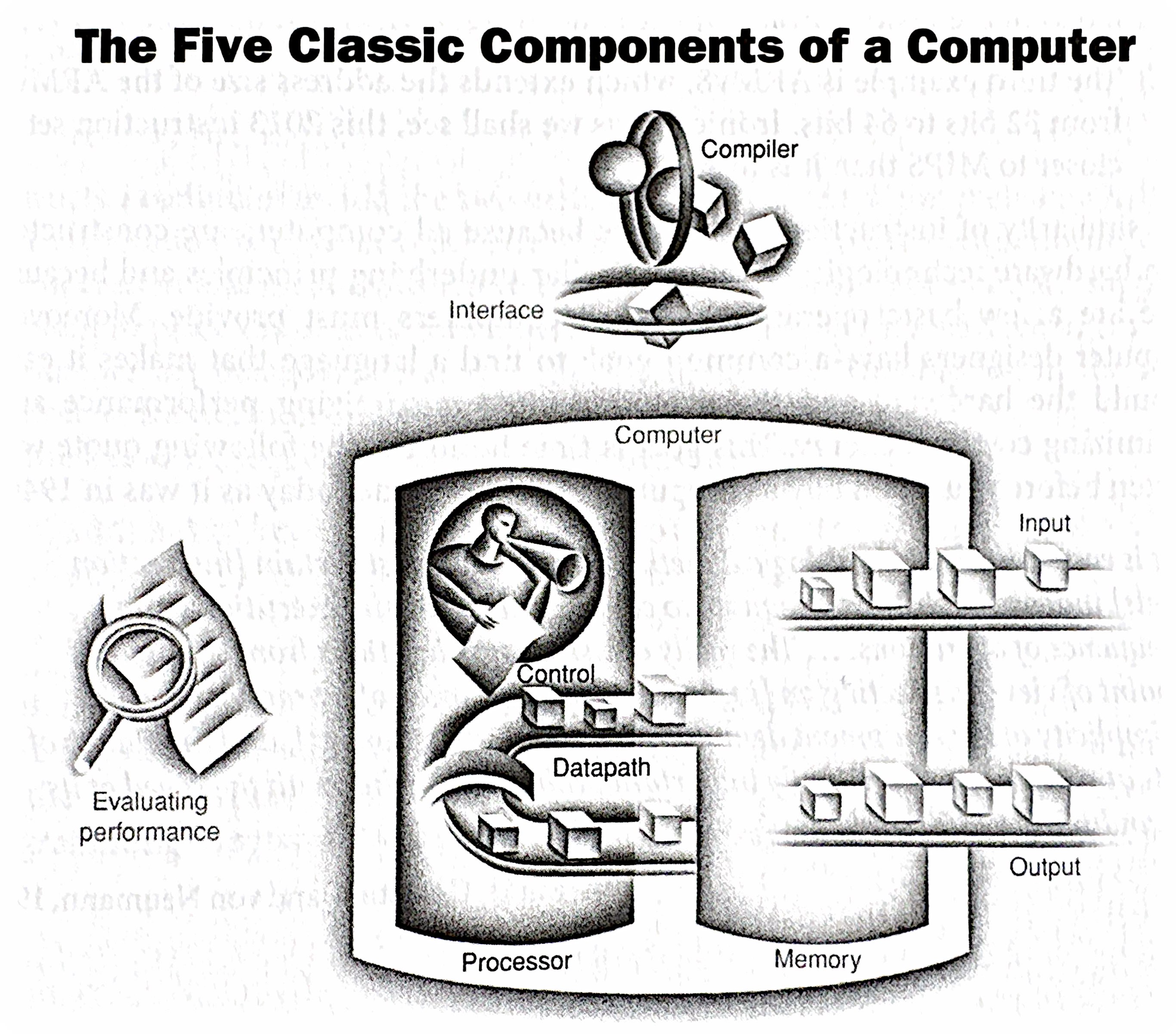
The Five Classic Components of a Computer
Every computer, from your smartphone to a supercomputer, can be conceptually broken down into five main components:
- Input: Mechanisms for feeding data into the computer (keyboard, mouse, network interface, sensors, etc.).
- Output: Mechanisms for displaying or transmitting results (monitor, printer, network interface, actuators, etc.).
- Memory: Stores both instructions (the program) and data that the computer is actively using. Think of it as the computer’s workspace. We’ll explore different types of memory (RAM, cache, registers) in detail later.
- Arithmetic Logic Unit (ALU): Performs the actual computations (arithmetic operations, logical comparisons) on the data. This is the “brain” of the CPU.
- Control Unit: Directs the operation of all other components. It fetches instructions from memory, decodes them, and issues signals to the ALU, memory, and I/O devices to execute those instructions. It’s the “conductor” of the computer’s orchestra.
These five components are interconnected by buses, which are sets of wires that carry data and control signals.
The Stored Program Concept
One of the most crucial concepts in computer architecture is the stored program concept. Before this, computers were often hardwired for specific tasks. Changing the program required rewiring the machine—a tedious and error-prone process.
The stored program concept, attributed to John von Neumann, revolutionized computing by storing both the instructions (the program) and the data in the computer’s memory. This allows for:
- Flexibility: Changing programs becomes as simple as loading a new set of instructions into memory.
- Automation: The computer can fetch and execute instructions sequentially without human intervention.
- Efficiency: Data and instructions can be accessed and manipulated quickly from memory.
This concept is fundamental to how all modern computers operate.
IV. von Neumann vs. Harvard Architectures
While the von Neumann architecture is dominant, it’s important to understand its historical context and alternatives.
| Feature | Von Neumann (Princeton) Architecture | Harvard Architecture |
|---|---|---|
| Memory | Single memory space for both instructions and data | Separate memory spaces for instructions and data |
| Access | Instructions and data share the same memory bus | Instructions and data can be accessed simultaneously |
| Advantages | Simpler design, more efficient use of memory | Faster instruction fetch, avoids bottlenecks |
| Disadvantages | Potential bottleneck (von Neumann bottleneck) as both instructions and data compete for the same memory access | More complex design, requires separate memory modules |
| Applications | General-purpose computers, PCs, laptops | Embedded systems, digital signal processors (DSPs) |
The von Neumann bottleneck arises because both instructions and data must travel over the same bus to and from memory. This can limit performance, especially when the CPU needs to fetch instructions and data frequently. The Harvard architecture mitigates this by allowing parallel access to instruction and data memories.
(Diagrams comparing the two architectures)
While modern general-purpose computers primarily use variations of the von Neumann architecture (often with caching and other techniques to reduce the bottleneck), the Harvard architecture is still relevant in specialized applications where performance and parallelism are critical.
Additional readings for these architecture types:
Introducing Performance of a Computer
Background reading on performance
Defining Performance in Computer Architecture
Performance in computer architecture is a multifaceted concept, and there isn’t one single “best” metric. It’s often a balancing act between different factors, and the “right” performance measure depends on the specific application and priorities. Here’s a breakdown of key aspects:
1. Execution Time:
- Definition: The most direct measure of performance is how long it takes a computer to complete a task. Shorter execution time means better performance.
- Units: Seconds, milliseconds, microseconds, etc.
- Factors: Clock speed, instruction count, memory access times, I/O speed, and overall system organization all influence execution time.
- Example: Comparing the time it takes two different processors to run the same benchmark program. The processor with the lower execution time is considered faster.
2. Throughput:
- Definition: Measures how much work a computer can complete in a given period. Higher throughput means better performance.
- Units: Transactions per second, jobs per hour, instructions per second (IPS), floating-point operations per second (FLOPS), etc.
- Factors: Processor core count, memory bandwidth, I/O bandwidth, and system software efficiency influence throughput.
- Example: A web server that can handle more requests per second has higher throughput. A supercomputer that can perform more FLOPS has higher computational throughput.
3. Latency:
- Definition: The delay between initiating a request and receiving the result. Lower latency means better performance.
- Units: Seconds, milliseconds, microseconds, nanoseconds, etc.
- Factors: Memory access times, network latency, disk access times, and pipeline stalls influence latency.
- Example: The time it takes for a mouse click to register on the screen is a measure of latency. A lower latency is crucial for interactive applications and real-time systems.
4. Resource Utilization:
- Definition: How efficiently a computer uses its resources (CPU, memory, I/O). Higher utilization (without bottlenecks) can lead to better performance.
- Units: Percentage of CPU usage, memory usage, disk I/O, etc.
- Factors: Operating system scheduling, memory management, and application design influence resource utilization.
- Example: A system that can perform the same amount of work using less energy or fewer CPU cycles is considered more efficient.
5. Power Consumption:
- Definition: The amount of energy a computer consumes. Lower power consumption is often desirable, especially in mobile and embedded systems. Performance per watt is a common metric.
- Units: Watts, milliwatts, kilowatts, etc.
- Factors: Processor architecture, clock speed, voltage, memory technology, and cooling systems influence power consumption.
- Example: A laptop that can run for longer on a single battery charge has better power efficiency.
- Note, the reading above speaks about the “Power Wall.” See below for additional notes on the power wall.
6. Cost:
- Definition: The price of the hardware and software. Performance per dollar is an important metric.
- Units: Dollars, etc.
- Factors: Processor cost, memory cost, storage cost
Sidebar — The Power Wall in Computer Architecture
The “Power Wall” refers to the increasing difficulty and impracticality of continuing to increase processor clock speeds to achieve performance gains. For many years, increasing clock speed was the primary driver of improved CPU performance. However, this approach has run into fundamental physical limitations, leading to the “power wall.”
The Problem:
As clock speeds increase, so does the power consumption of the processor. This increased power consumption manifests as heat. The relationship is roughly cubic: doubling the clock speed can increase power consumption by a factor of eight. This heat becomes increasingly difficult and expensive to dissipate. Think of it like trying to cool a rapidly boiling pot of water; at some point, you can’t add any more heat without it boiling over.
Consequences of Excessive Heat:
- Reliability Issues: High temperatures can damage components and reduce the lifespan of the processor.
- Cooling Costs: More complex and expensive cooling solutions (e.g., liquid cooling) are required to manage the increased heat. This adds to the overall system cost.
- Power Consumption: Higher power consumption translates to higher energy bills and reduces battery life in mobile devices. This has significant environmental implications as well.
- Diminishing Returns: At a certain point, the performance gains from increasing clock speed are outweighed by the increased power consumption and cooling costs. The extra heat generated becomes unmanageable, and further increases in clock speed provide only marginal performance improvements.
The Relationship Between Clock Speed and Power
- Dynamic Power: A significant portion of a processor’s power consumption is dynamic power, which is the power used to switch transistors on and off. This is directly related to the clock speed. Note there is also “static power consumption,” also known as the leakage current to power up transitors. We will deal here only with dynamic power, that is, the power created by switching between 0s and 1s.
- The Equation: Power is that generated when switching between 0 and 1 and the static power: \(P=P_{dynamic}+P_{static}\) where $P_{dynamic} = C * V^2 * f$.
A simplified way to represent this is: \(Power ≈ C * V^2 * f\)
Where:
Cis the capacitance of the circuitVis the voltage-
fis the frequency (clock speed) - The Cube Relationship: Notice that the voltage (
V) is squared in this equation. This is crucial. To increase clock speed, you often need to increase the voltage to maintain stability. This means that the power increases quadratically with voltage. Since voltage often needs to be increased proportionally with frequency, you end up with a cubic relationship overall.
Why It’s Close to a Factor of Eight
- Linear Increase with Frequency: If you only doubled the clock speed and kept the voltage the same, the power would increase linearly (doubling).
- Voltage Increase: However, to reliably double the clock speed, you typically need to increase the voltage. This increase in voltage, when squared, has a much larger impact on power consumption.
- Combined Effect: The combination of the linear increase from frequency and the quadratic increase from voltage results in a power increase that is close to a factor of eight when you double the clock speed.
Important Caveats
- Technology Nodes: As semiconductor technology advances, the relationship between clock speed and power becomes more complex. New techniques and materials can help mitigate the power increase.
- Design Techniques: Architects use various techniques (like clock gating, power gating, and voltage scaling) to manage power consumption and improve efficiency.
- Leakage: In modern processors, leakage current (current that flows even when a transistor is off) also contributes to power consumption, and this can become more significant at higher temperatures associated with higher clock speeds.
In Summary
While not an absolute rule, the “factor of eight” is a good rule of thumb to illustrate the significant power challenges associated with increasing clock speeds. It highlights the need for innovative design techniques and power management strategies in modern computer architecture.
The Shift in Focus:
The power wall has forced a fundamental shift in how computer architects design processors. Instead of focusing solely on increasing clock speed, the emphasis has moved towards:
- Multi-core Processors: Instead of one fast core, processors now have multiple slower cores that can work in parallel. This allows for increased throughput without dramatically increasing power consumption.
- Specialized Hardware: Adding specialized hardware units for specific tasks (e.g., graphics processing units (GPUs), digital signal processors (DSPs)) can improve performance without increasing the clock speed of the main processor.
- Architectural Innovations: Developing new microarchitectural techniques, such as pipelining, caching, and branch prediction, can improve performance without relying solely on higher clock speeds.
- Power-Efficient Designs: Designing processors with lower voltage and more efficient transistors can reduce power consumption.
- Dark Silicon: The idea that not all transistors on a chip can be powered on at the same time due to thermal constraints. This necessitates intelligent power management strategies.
In summary: The power wall is a critical challenge in computer architecture. It signifies the limitations of simply increasing clock speeds to achieve performance gains. The industry has responded by shifting its focus towards multi-core processors, specialized hardware, architectural innovations, and power-efficient designs. Managing power consumption and heat dissipation has become a central concern for computer architects.
Looking Ahead to next lecture — Instruction Set Architecture (ISA)
Today, we’ve laid the foundation for understanding the basic components and principles of computer architecture. Our next lecture will delve into the Instruction Set Architecture (ISA).
The ISA defines the set of instructions that a particular processor can understand and execute. It’s the interface between the hardware and the software. We’ll explore:
- Instruction formats: How instructions are encoded and represented in memory.
- Addressing modes: How the processor accesses data in memory.
- Instruction types: Arithmetic, logical, data transfer, control flow, etc.
- ISA design considerations: How ISA choices impact performance, complexity, and programmability.
Understanding the ISA is crucial for writing efficient code, optimizing compiler design, and designing new processors. It’s the bridge between the high-level world of programming and the low-level world of hardware.